Solving the heat equation

In this notebook we will learn how to use tensorized linear solvers for solving a partial differential equation (PDE). The PDE in question will be the heat equation \(\Delta x = b\). \(\Delta\) is the laplace operator and \(b\) some boundary condition. We will solve the equation in question with finite difference on a two dimensional grid.

import numpy as np
from trainsum.numpy import trainsum as ts
from trainsum.typing import UniformGrid
import matplotlib.pyplot as plt

def laplace(grid: UniformGrid, idx: int) -> ts.TensorTrain[NDArray]:
    """
    Get the tensor train which represents the finite difference
    laplace operator with the dimension defined by idx.
    """
    train = None
    with ts.exact():
        for i, dim in enumerate(grid.dims):
            if i == idx:
                tmp  = -2.0 * ts.shift(dim, 0)
                tmp +=  1.0 * ts.shift(dim, -1)
                tmp +=  1.0 * ts.shift(dim, 1)
                tmp *= -1/grid.spacings[0]**2
            else:
                tmp = ts.shift(dim, 0)
            if train is None:
                train = tmp
            else:
                train.extend(tmp)
    return train

As a first step we define the laplace operator as a tridiagonal toeplitz matrix with -2 on the main diagonal and 1 on the diagonals above and below.

# define the domain on which the problem is solved
shape = ts.trainshape(32, 32, mode="block")
domains = ts.domain(0.0, 1.0), ts.domain(0.0, 1.0)
grid = ts.uniform_grid(shape.dims, domains)

xshape = ts.trainshape(shape.dims[0])
yshape = ts.trainshape(shape.dims[1])

Next we define solution space with an uniformly spaced grid. For doing so we will need some dimensions which are associated to some intervals (domains).

# create a tensor train, which has ones at one side else zeros
with ts.variational(max_rank=1):
    data = np.zeros(shape.dims[0].size())
    data[0] = 1.0
    rhs = ts.tensortrain(xshape, data)
    rhs.extend(ts.full(yshape, 1))

# multiply the train along the y-axis with a gauss-shapes function
with ts.variational(max_rank=10):
    y = np.linspace(domains[1].lower, domains[1].upper, shape.dims[1].size())
    data = np.exp(-10*(y-0.5)**2) # change this part to get another boundary condition
    #data =  (y-0.5)**2
    tmp = ts.tensortrain(yshape, data)
    rhs = ts.einsum("ab,b->ab", rhs, tmp)

# plot the resulting matrix
plt.figure()
plt.imshow(rhs.to_tensor())
plt.show()

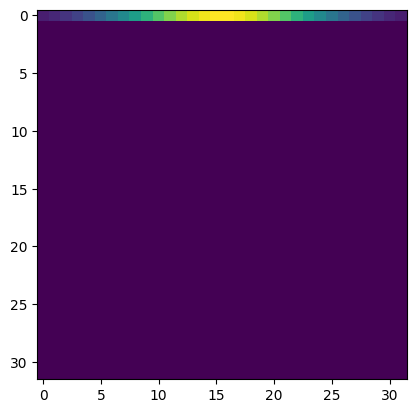
In the next cell we define the boundary condition \(b\). It is chosen so one site of the square represents a gaussian shaped function.

# define the laplace operators
shape.ranks = 15
laplace_ops = [laplace(grid, i) for i in range(len(shape.dims))]
laplace_maps = [ts.linear_map("imjn,mn->ij", op, shape) for op in laplace_ops]

After defining the right hand side of the equation we will see how to define the linear operators used to define the linear equation system. Since \(\Delta\) is the sum of its \(x\) and \(y\) component, we can define it as two seperate operators \(\Delta_x\) and \(\Delta_y\).

# define the strategy and local solvers
strat = ts.sweeping_strategy(ncores=2, nsweeps=5)
decomp = ts.svdecomposition(max_rank=10, cutoff=1e-6)
solver = ts.gmres(nsteps=25, subspace=25, eps=1e-6)

# define the tensorized linear solver
lin_solver = ts.linsolver(
    rhs,
    *laplace_maps,
    method="dmrg",
    strategy=strat,
    decomposition=decomp,
    solver=solver)

At this step all components of the equation are defined and we can instantiate the solver. For doing so we need a sweeping strategy, a decomposition (for strategies with ncores >= 2) and a non tensorized solver for linear equation systems. Since it is very convenient to implicitly define the local linear maps the library implements a GMRES solver.

# callback for printing and retrieval of local results
vals = []
def callback(lrange, res):
    print(f"{res.residuals[-1]:.8E}", end="\r", flush=True)
    vals.append(res.residuals[-1])
    return False

# create some start guess and solve the system
guess = ts.full(shape, 1)
res = lin_solver(guess, callback=callback)

7.08044032E-07

With the solver we can now start the process of solving the equation.

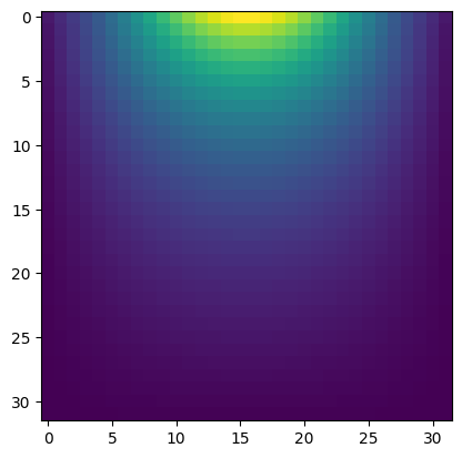
# plot the heat map
plt.figure()
plt.imshow(res.to_tensor())
plt.show()