Getting Started
Installation
trainsum can be installed via pip.
pip install trainsum
- The dependencies are:
numpy
array_api_compat
opt_einsum
h5py
pulp[cbc] (you might want to install GLPK for better performance)
Importing the library
The public API of trainsum is provided by the TrainSum class.
Three backends are supported out of the box:
from trainsum.numpy import trainsum as ts
from trainsum.cupy import trainsum as ts
from trainsum.torch import trainsum as ts
Since the package uses internally the Array API standard one can also use another compatible library.
TrainSum expects the library to have mutable N-dimensional arrays with shapes that are defined at all times (which rules out JAX or Dask).
Quantized dimensions
Having imported the library we can start with the most important concept, the quantized dimension. A quantized dimension is a dimension of size N, which has been factorized into some integers, referred to as digits. With trainsum this can be simply done via
dim = ts.dimension(20),
where \(20\) is factorized into \(2\cdot 2\cdot 5\cdot\) using the prime factorization.
We can also explicitly specify the factorization by passing a list of integers to dimension()
dim = ts.dimension([2, 5, 2])
A Dimension is a sequence of Digit instances, which hold the integers of the factorization.
TrainShape
The next concept is the shape of a tensor train which is expressed through the class TrainShape.
It is defined as a sequence of grouped Digit instances.
The sequence is not unique and can be chosen arbitrarily as long as all digits of a dimension, which is part of the train, are used.
The preferred way of defining a TrainShape is with the trainshape() function.
from trainsum.numpy import trainsum as ts

shape = ts.trainshape(20)

dims = ts.dimension(20), 36
block_shape = ts.trainshape(*dims, mode='block')

dims = ts.dimension(20), ts.dimension(36)
interleaved_shape = ts.trainshape(*dims, mode='interleaved')
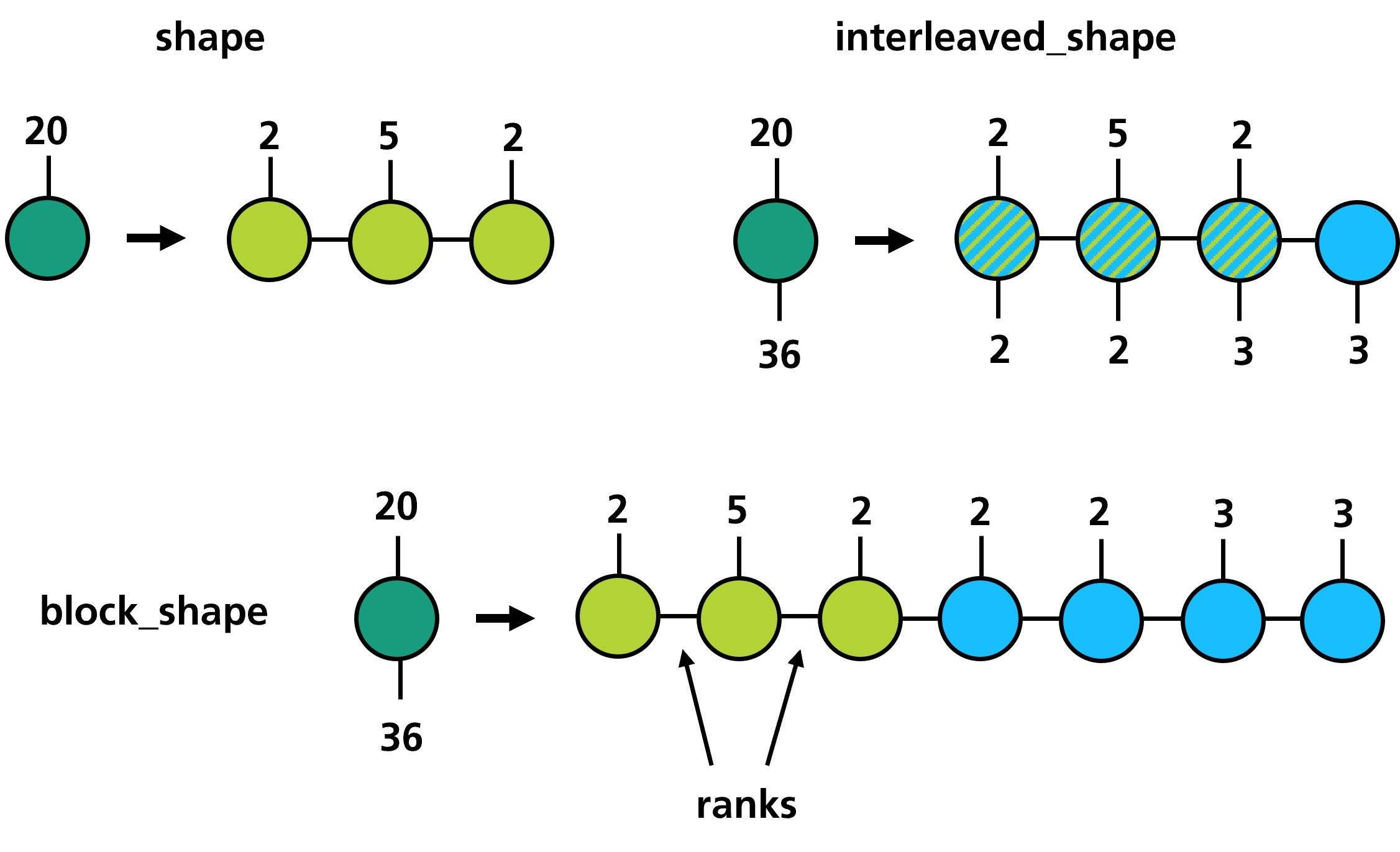
TrainShape does not only define the arrangement of the digits within the tensor train but also the size of the internal dimensions.
These dimensions are often called bond dimensions and the corresponding sizes are called ranks.
Construction
Using the shape of a tensor train we can finally turn towards the construction, which can be done in multiple ways. One way is the explicit construction of functions that have a well defined tensorized structure. This includes:
functions, where all values are the same
exponentials
cosine and sine
polynomials
shift matrices
Toeplitz tensors
discrete Fourier-transformations
For some of those we need a UniformGrid, which can be initialized with a Dimension and a Domain.
from trainsum.numpy import trainsum as ts

dim = ts.dimension(1024)
domain = ts.domain(-1.0, 1.0)
grid = ts.uniform_grid(dim, domain)

train = ts.sin(grid, 1.0, 0.0)               # sin( 1.0 * (x-0.0) )
train = ts.polyval(grid, [1.0, 0.0, 0.0], 0.5)  # (x-0.5)^2
Another way of defining tensor trains is with the tensortrain() function.
The first argument of tensortrain() is always a TrainShape.
The second argument can either be a full tensor or a function.
In that case the tensor or the function are converted to a tensor train.
If the second argument is a sequence of tensors, the tensors are interpreted as the tensor cores of the tensor train.
import numpy as np
from trainsum.numpy import trainsum as ts

shape = ts.trainshape(1024)
domain = ts.domain(-1.0, 1.0),
grid = ts.uniform_grid(shape.dims, domain)

# data approximation
data = np.linspace(-1.0, 1.0, 1024)**2
train = ts.tensortrain(shape, data)

# function approximation
func = lambda idxs: np.exp(-np.sum(grid.to_coords(idxs)**2, axis=0))
train = ts.tensortrain(shape, func)

# explicit construction with cores
cores = [np.ones([1, digit.base, 1]) for digit in shape.dims[0]]
train = ts.tensortrain(shape, cores)
Arithmetic
The arithmetic of tensor networks is not at all straightforward and uses multiple algorithms and methods. Some arithmetic operations like addition or matrix multiplication can be performed exactly within the numerical precision. Doing so leads to a increase of the ranks and may lead to tensor trains that do not have a computational advantage. To counteract the increasing ranks we can perform the operations approximately using either decomposition (also called zip-up) algorithms or variational algorithms. A lot of other operations, especially element wise operations, like abs or sqrt cannot be performed exactly. The fallback in these cases is a sampling algorithm, the cross interpolation.
The main functions for arithmetic operations are einsum(), einsum_expression(), add(), transform() and the magic methods of the TensorTrain class like __mul__.
To easily define the corresponding algorithms in the background trainsum heavily relies upon context managers.
There are five of them available:
context manager |
affects |
|---|---|
exact |
einsum, addition, multiplication |
decomposition |
einsum, addition, multiplication, tensortrain (with data) |
variational |
einsum, addition, multiplication, tensortrain (with data) |
cross |
TensorTrain transformations, tensortrain (with function) |
evaluation |
TensorTrain transformations, tensortrain (with function), evaluations |
import numpy as np
from trainsum.numpy import trainsum as ts

shape = ts.trainshape(1024)

# data approximation
data1 = np.linspace(-1.0, 1.0, 1024)**2
train1 = ts.tensortrain(shape, data1)

data2 = np.exp(-np.linspace(-1.0, 1.0, 1024)**2)
train2 = ts.tensortrain(shape, data2)

# einsum operations
with ts.decomposition(max_rank=5, cutoff=1e-10, ncores=2): # or ts.exact/ts.variational
    res = train1 * train2
    train1 += train2
    res = ts.einsum('i,i->i', train1, res)

# element-wise operation
with ts.cross(max_rank=16, eps=1e-10), ts.evaluation(chunk_size=1024):
    res = train1.transform(lambda x: x**0.5)
The context managers are stored in a global dictionary with (backend, option_type, threading_id) as key and delete themselves upon calling their exit function.
One can globally set the options via set_options().
Solvers
trainsum provides solvers for eigenvalue equations and linear equation systems.
The solvers are defined by linear operators (linear_map()), that can be defined with einsum-like expressions.
Here is an example for solving the quantum harmonic oscillator:
from trainsum.numpy import trainsum as ts

# define the settings
shape = ts.trainshape(1024)
domain = ts.domain(-10.0, 10.0),
grid = ts.uniform_grid(shape.dims, domain)

# create the laplace operator
dim = shape.dims[0]
with ts.exact():
    laplace = -2*ts.shift(dim, 0)
    laplace += ts.shift(dim, 1)
    laplace += ts.shift(dim, -1)
    laplace *= -0.5/grid.spacings[0]**2
laplace_map = ts.linear_map("ij,j->i", laplace, shape)

# create the potential operator
pot = ts.polyval(grid, [1.0, 0.0, 0.0], 0.0)
pot_map = ts.linear_map("i,i->i", pot, shape)

# define the options of the eigsolver
decomp = ts.svdecomposition(max_rank=15, cutoff=1e-10)
strat = ts.sweeping_strategy(ncores=2, nsweeps=10)
loc_solver = ts.lanczos()

# get the solver instance
solver = ts.eigsolver(
    laplace_map, pot_map,
    decomposition=decomp,
    strategy=strat,
    solver=loc_solver)

# create an initial guess and solve the problem
guess = ts.full(shape, 1.0)
res = solver(guess)
Further steps
Some applications and potential use cases are shown as Jupyter notebooks in the Examples chapter.