Convolution

In this notebook we will see how to perform discrete convolutions using the Toeplitz tensor.

import numpy as np
from trainsum.numpy import trainsum as ts
import matplotlib.pyplot as plt

opts = ts.variational(max_rank=10, cutoff=1e-10)
ts.set_options(opts)

opts = ts.cross(max_rank=20, eps=0.0)
ts.set_options(opts)

First we set some global options so we do not need context manager for every operation

# define the problem domain
dim = ts.dimension(1024)
shape = ts.trainshape(1024)
domain = ts.domain(0, 1)
grid = ts.uniform_grid(dim, domain)

The first example will be one dimensional so we define a simple uniformly spaced 1D grid with 1024 points.

# create a square and exponential function
square = (ts.shift(dim, -256)) @ (ts.shift(dim, 2*256) @ ts.full(shape, 1.0))
exp = ts.shift(dim, -256) @ ts.exp(grid, -10.0, 0.0)

# visualize the functions
fig, ax = plt.subplots(ncols=2, figsize=(12, 4))
ax[0].plot(square.to_tensor())
ax[0].grid()
ax[1].plot(exp.to_tensor())
ax[1].grid()
plt.show()

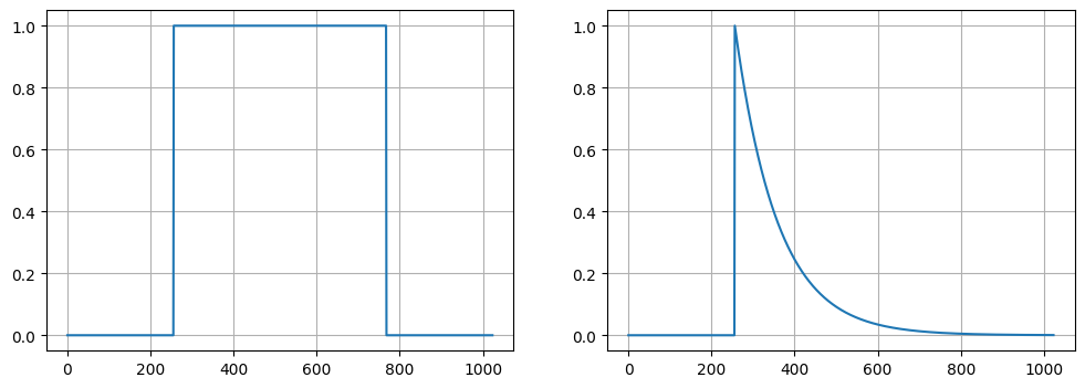
Having defined the grid we can define two simple function that are textbook examples for explaining a convolution. On the left we have a simple square function. On the right is a exponential decay of some kind.

# create the convolution operator
toeplitz = ts.toeplitz(dim, mode="full")

# apply the convolution operator
res = ts.einsum("ijk,j,k->i", toeplitz, exp, square)

# calculate the reference
ref = np.convolve(square.to_tensor(), exp.to_tensor())

# plot the results
plt.figure(figsize=(6,4))
plt.plot(ref)
plt.plot(res.to_tensor(), linestyle="dashed")
plt.grid()
plt.show()

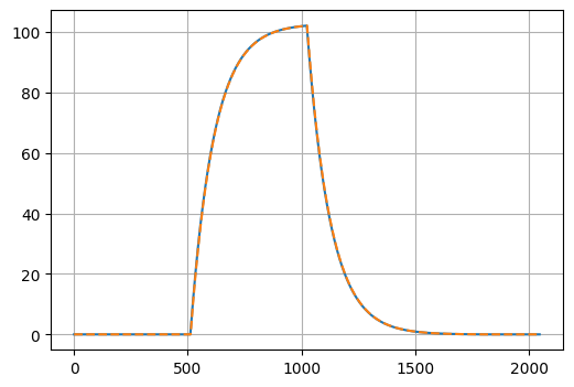
In this cell we construct the 3D toeplitz tensor with rank=2. After that we use the einstein summation “ijk,j,k->i” to perform the convolution. Finally we compare the result against NumPy’s convolve function.

# define the problem domain
shape = ts.trainshape(1024, 1024)
dims = shape.dims
domains = ts.domain(-10, 10), ts.domain(-10, 10)
grid = ts.uniform_grid(dims, domains)

Next we want to perform a 2D convolution, so we create a 2D grid.

#create a picture with a square
train = ts.full(shape, 1.0)
op = ts.shift(dims[0], -256) @ ts.shift(dims[0], 2*256)
train = ts.einsum("ij,jk->ik", op, train)
train = ts.einsum("ij,kj->ki", op, train)

# learn the gaussian kernel
func = lambda idxs: np.exp(-0.2*np.sum(grid.to_coords(idxs)**2, axis=0))
kernel = ts.tensortrain(shape, func)

# plot the picture and the guassian kernel
fig, ax = plt.subplots(ncols=2, figsize=(15, 4))
ax[0].imshow(train.to_tensor())
ax[1].imshow(kernel.to_tensor())
plt.show()

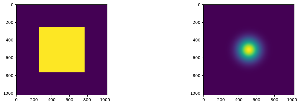
Using the 2D grid we define a square function and a gaussian-shaped function.

# create the convolution operator
toeplitz = ts.toeplitz(dims[0], mode="full")
toeplitz.extend(ts.toeplitz(dims[1], mode="full"))

# apply the convolution operator
res = ts.einsum("ijkmno,jn,ko->im", toeplitz, train, kernel)

# plot the result
plt.figure()
plt.imshow(res.to_tensor())
plt.show()

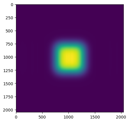
Finally we create a multilevel Toeplitz matrix by calculating the outer product of two normal Toeplitz matrices (using the extend method). After doing so we write down the correct einsum expression and execute it.